Computing the DFC/HP and manipulating the functions returned objects
Hassan-Roland Nasser and Marie Schneider
2025-03-11
DFC_and_HP_and_changing_plots.Rmd
library(digiRhythm)
data <- digiRhythm::df691b_1
data <- resample_dgm(data, 15)
data <- remove_activity_outliers(data)
activity <- names(data)[3]
head(activity)
#> [1] "Steps"
Degree of Functional Coupling (DFC) and Harmonic Power (HP)
The degree of functional coupling and the harmonic power could be computed using the dfc function as shown below.
The DFC algorithm is a bit complicated. It’s, therefore, needed that we clarify few points about some computing considerations and also about the arguments of the function itself:
- The recommended sampling period is between 15 and 30 min.
- The DFC and HP are computed each X days. We call X the rolling window. For example, if the rolling window is 7 days, the first DFC/HP value is computed for the subset between day 1 and day 7, and the second DFC/HP value is computed for the subset between day 2 and day 8, and so on. If the data contains 8 days of data, then we will only have two DFC and HP values. The recommended rolling window is 7 days, however the user can choose a rolling window not less than two days and not more that the number of days in the dataset -1.
- As the computation of DFC/HP are mainly based on the power of the 24-hours harmonics (24/1 is the first harmonic, 24/2 is the second harmonic, 24/3 is the third harmonic, and so on), the user can choose up till which harmonic to consider. The default value is 12. It’s important to note that the lowest harmonic period should be twice bigger than the sampling period. For example, if your data is sampled at 15 minutes, then the lowest harmonic period should be 30 minutes. This is because the Nyquist frequency is half the sampling frequency. Consequently, the harmonic cutoff parameter should be set to not more than 48 (because 24 hours * 60 min / 48 = 30 min = 2 * 15 min of sampling period).
The user does not need to worry about looping over days or extracting the Lomb Scargle periodogram for every X (rolling window) days and then compile the results to obtain the degree of functional coupling. This is done in loop inside the dfc function. However, there is also a function call lomb_scargle_periodogram where the user can investigate the activity a little bit deeper. We preview the lomb_scargle_periodogram function and its output, then we go to the dfc function.
df <- data[1:672, c("datetime", activity)]
my_lsp <- lomb_scargle_periodogram(df, alpha = 0.01, plot = TRUE)
#> v Correct time format: First column has a POSIXct Format
#> v Number of days good for DFC: 8 days >= 2 days
#> v Correct numeric format - Column 2 ==> Steps
#> The data is digiRhythm friendly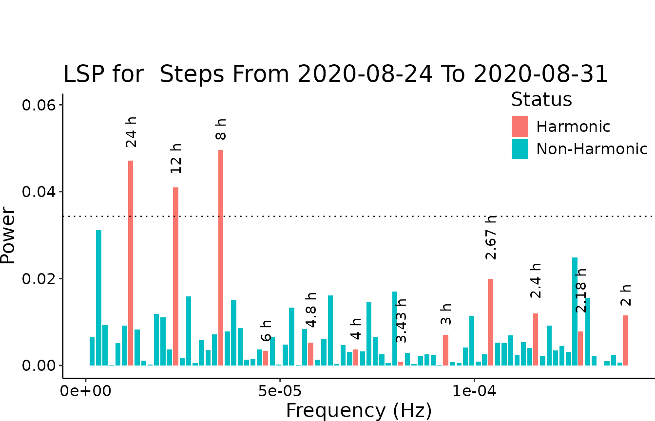
In the above plot, we see plenty of information. First, we have the whole periodogram for the dataframe df visualized. Second, we can distinguish between harmonic and non harmonic frequencies. Harmonic frequencies are plotted in blue and tagged with the time period they correspond to. For instance, we can check the power of the 24h cycles, 12h cycles, 6h cycles and so on. Third, we have a dotted horizontal line that makes it easy to visually check which frequencies are considered to originated from noise rather than from a actual signal. Frequency bars that make it above this line are considered to be originated from a real activity. The probability of this event is calculated using the method of Baluev (2008). The plot also shows, as title, the activity time span used for the computation. Warning: At the moment, function only computes the LSP the first 7 days of the data. A loop, to calculate LSP for the whole data, will be included in a later version. However, at the moment user can see the LSP-diagrams of the whole data, if running the dfc function. Before the complete DFC and HP diagram, each LSP diagram of the sliding 7-day periods were computed.
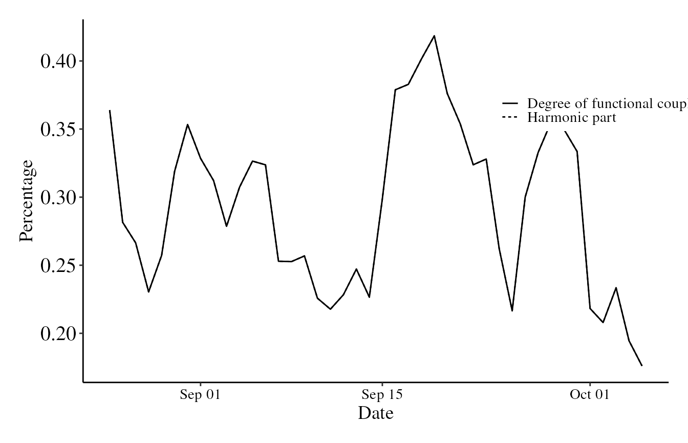
Now, to the DFC. The below plot shows the DFC and HP in the same graph. Both variables are percentages.
my_dfc <- dfc(data, # The dataset
  activity = activity, # the name of the activity column
  sampling = 15, # the sampling frequency of my dataset is 15
  alpha = 0, 5, # significance level
  harm_cutoff = 12, # up till the harmonic 24/12 which is two hours
  plot = FALSE, verbose = FALSE
)
#>              datetime Motion.Index Steps
#> 1 2020-08-25 00:00:00           20     8
#> 2 2020-08-25 00:15:00           52    46
#> 3 2020-08-25 00:30:00           61    39
#> 4 2020-08-25 00:45:00           29    18
#> 5 2020-08-25 01:00:00           83    26
#> 6 2020-08-25 01:15:00           50    23
#> [1] 43
#> v Correct time format: First column has a POSIXct Format
#> v Number of days good for DFC: 4 days >= 2 days
#> v Correct numeric format - Column 2 ==> Steps
#> The data is digiRhythm friendly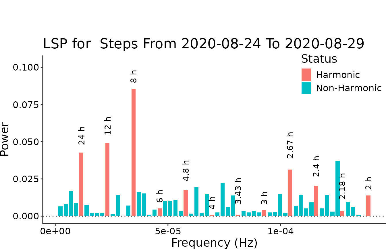
#> v Correct time format: First column has a POSIXct Format
#> v Number of days good for DFC: 5 days >= 2 days
#> v Correct numeric format - Column 2 ==> Steps
#> The data is digiRhythm friendly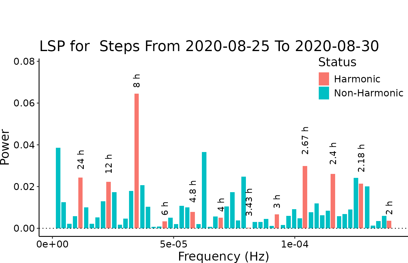
#> v Correct time format: First column has a POSIXct Format
#> v Number of days good for DFC: 5 days >= 2 days
#> v Correct numeric format - Column 2 ==> Steps
#> The data is digiRhythm friendly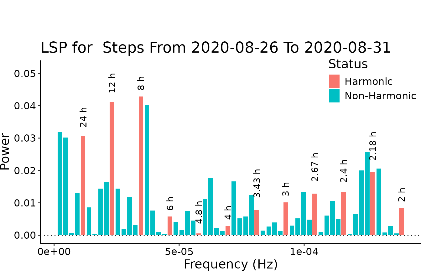
#> v Correct time format: First column has a POSIXct Format
#> v Number of days good for DFC: 5 days >= 2 days
#> v Correct numeric format - Column 2 ==> Steps
#> The data is digiRhythm friendly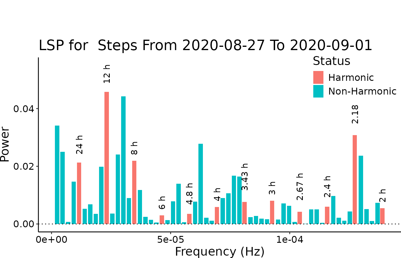
#> v Correct time format: First column has a POSIXct Format
#> v Number of days good for DFC: 5 days >= 2 days
#> v Correct numeric format - Column 2 ==> Steps
#> The data is digiRhythm friendly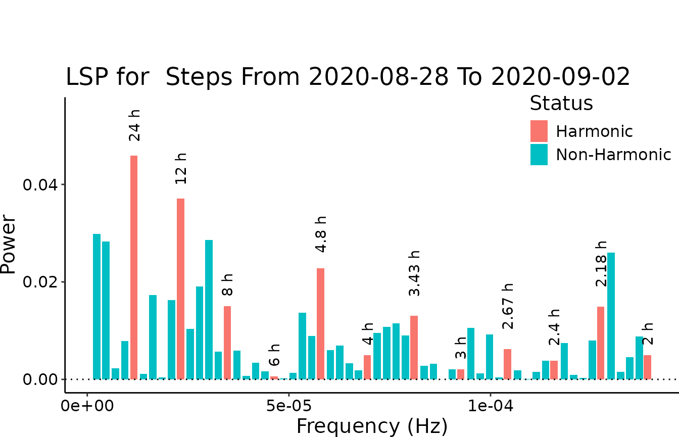
#> v Correct time format: First column has a POSIXct Format
#> v Number of days good for DFC: 5 days >= 2 days
#> v Correct numeric format - Column 2 ==> Steps
#> The data is digiRhythm friendly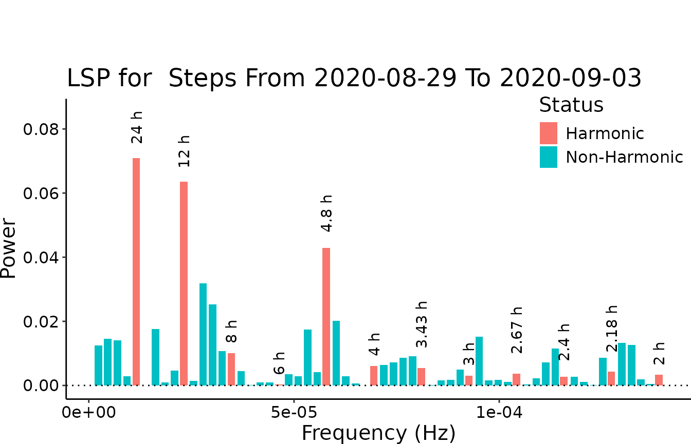
#> v Correct time format: First column has a POSIXct Format
#> v Number of days good for DFC: 5 days >= 2 days
#> v Correct numeric format - Column 2 ==> Steps
#> The data is digiRhythm friendly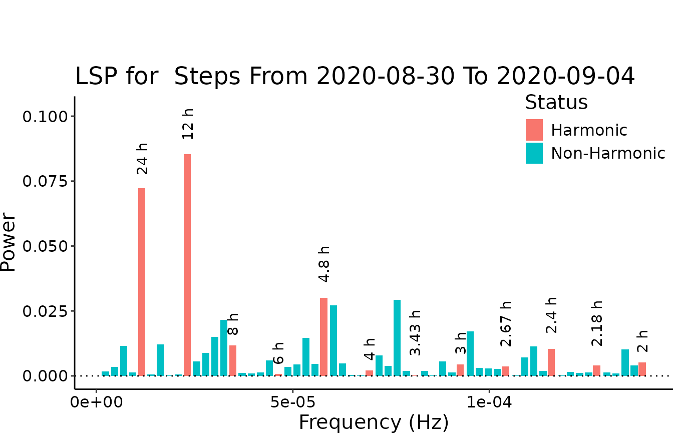
#> v Correct time format: First column has a POSIXct Format
#> v Number of days good for DFC: 5 days >= 2 days
#> v Correct numeric format - Column 2 ==> Steps
#> The data is digiRhythm friendly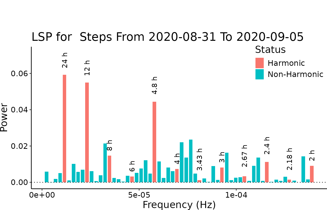
#> v Correct time format: First column has a POSIXct Format
#> v Number of days good for DFC: 5 days >= 2 days
#> v Correct numeric format - Column 2 ==> Steps
#> The data is digiRhythm friendly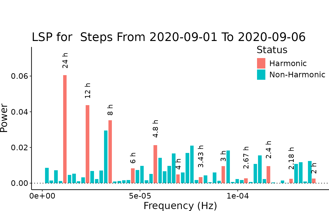
#> v Correct time format: First column has a POSIXct Format
#> v Number of days good for DFC: 5 days >= 2 days
#> v Correct numeric format - Column 2 ==> Steps
#> The data is digiRhythm friendly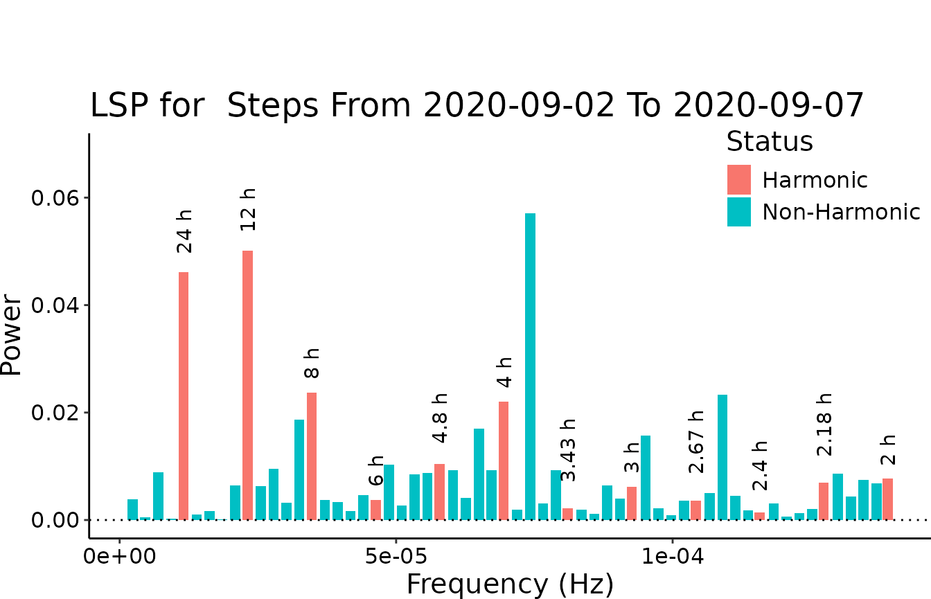
#> v Correct time format: First column has a POSIXct Format
#> v Number of days good for DFC: 5 days >= 2 days
#> v Correct numeric format - Column 2 ==> Steps
#> The data is digiRhythm friendly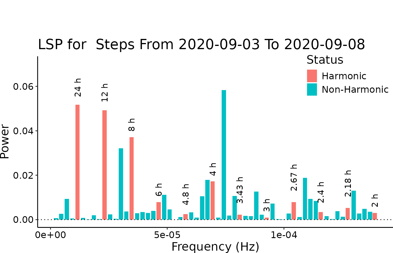
#> v Correct time format: First column has a POSIXct Format
#> v Number of days good for DFC: 5 days >= 2 days
#> v Correct numeric format - Column 2 ==> Steps
#> The data is digiRhythm friendly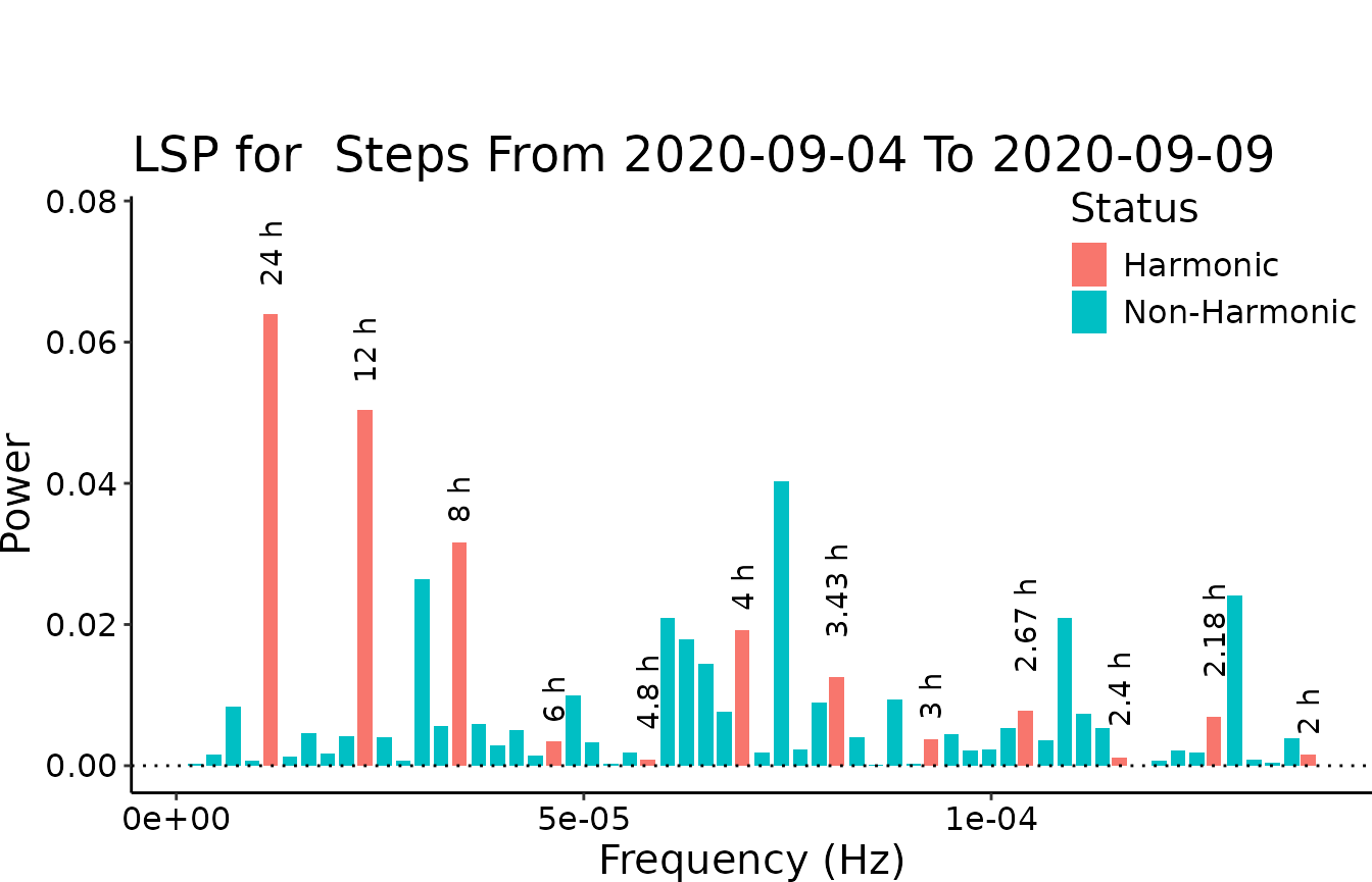
#> v Correct time format: First column has a POSIXct Format
#> v Number of days good for DFC: 5 days >= 2 days
#> v Correct numeric format - Column 2 ==> Steps
#> The data is digiRhythm friendly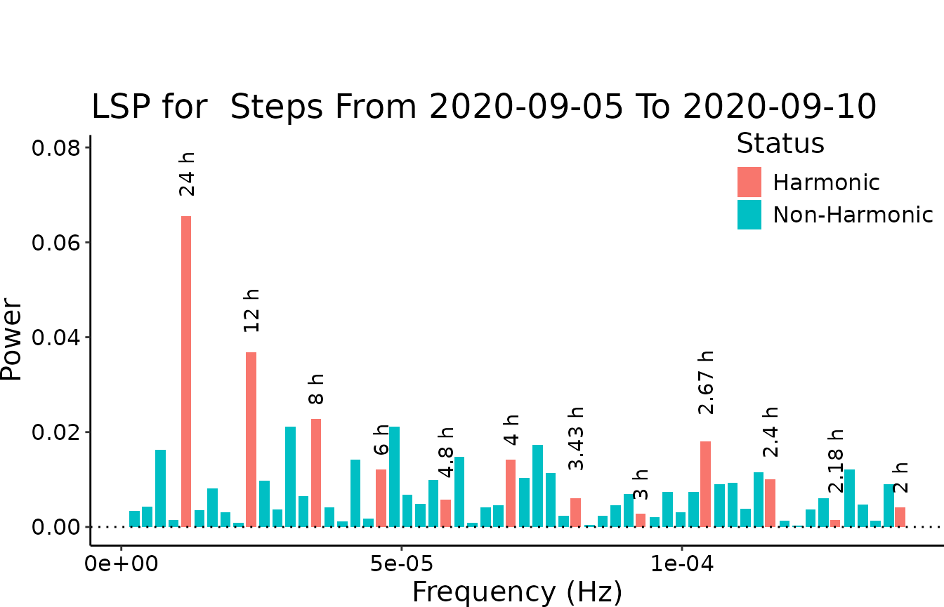
#> v Correct time format: First column has a POSIXct Format
#> v Number of days good for DFC: 5 days >= 2 days
#> v Correct numeric format - Column 2 ==> Steps
#> The data is digiRhythm friendly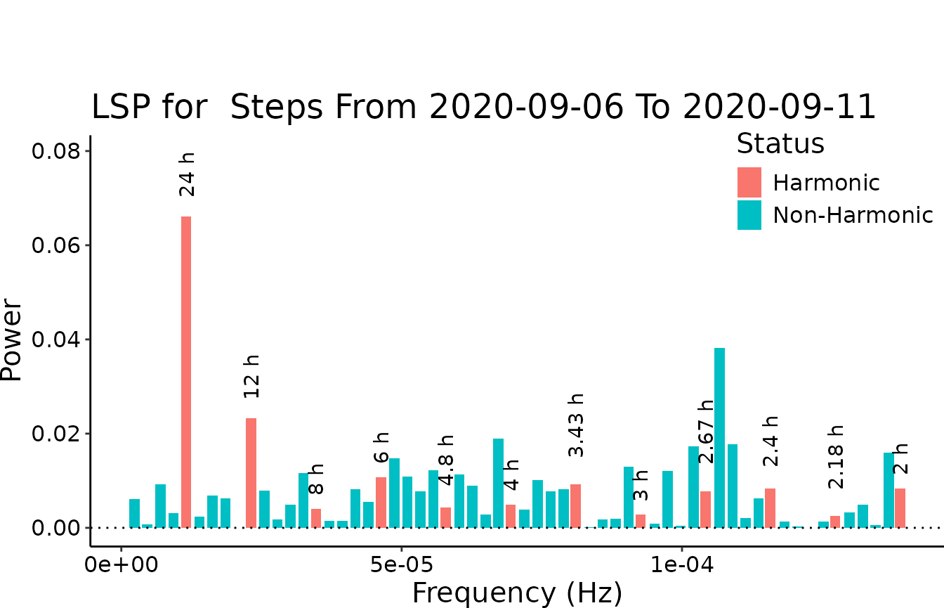
#> v Correct time format: First column has a POSIXct Format
#> v Number of days good for DFC: 5 days >= 2 days
#> v Correct numeric format - Column 2 ==> Steps
#> The data is digiRhythm friendly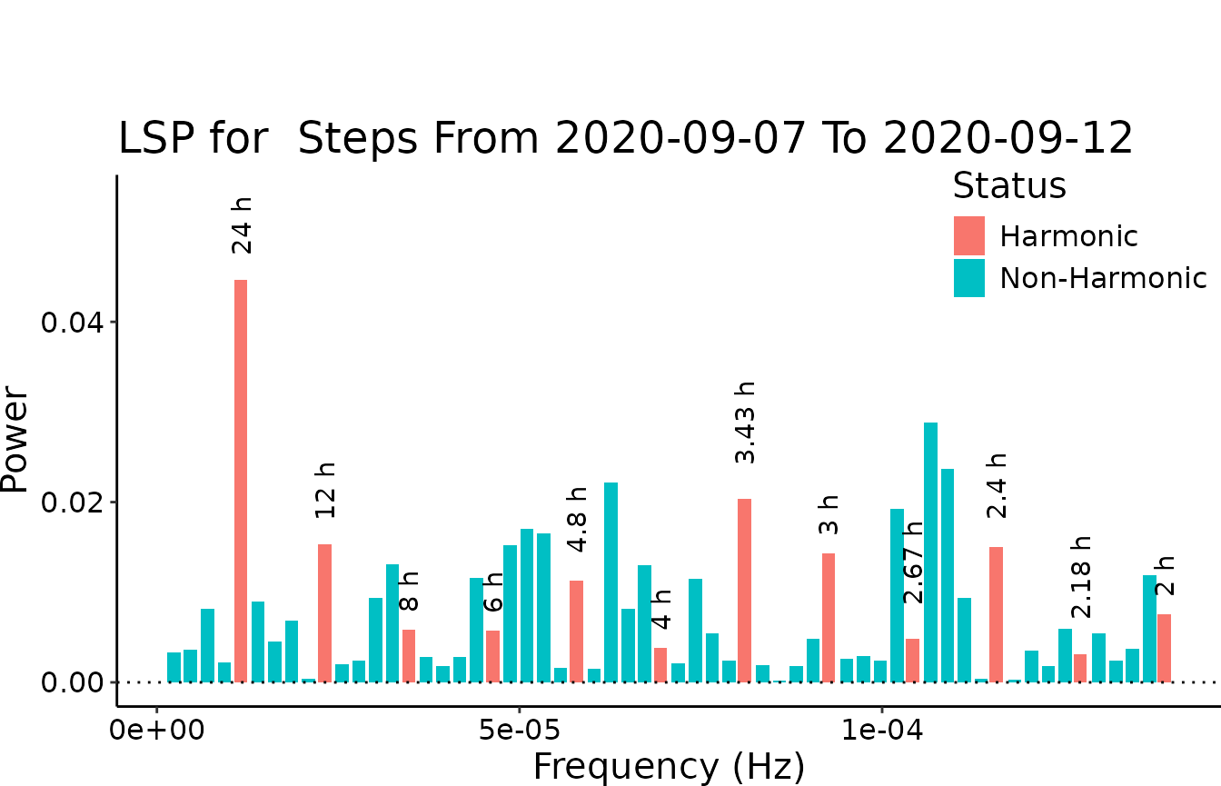
#> v Correct time format: First column has a POSIXct Format
#> v Number of days good for DFC: 5 days >= 2 days
#> v Correct numeric format - Column 2 ==> Steps
#> The data is digiRhythm friendly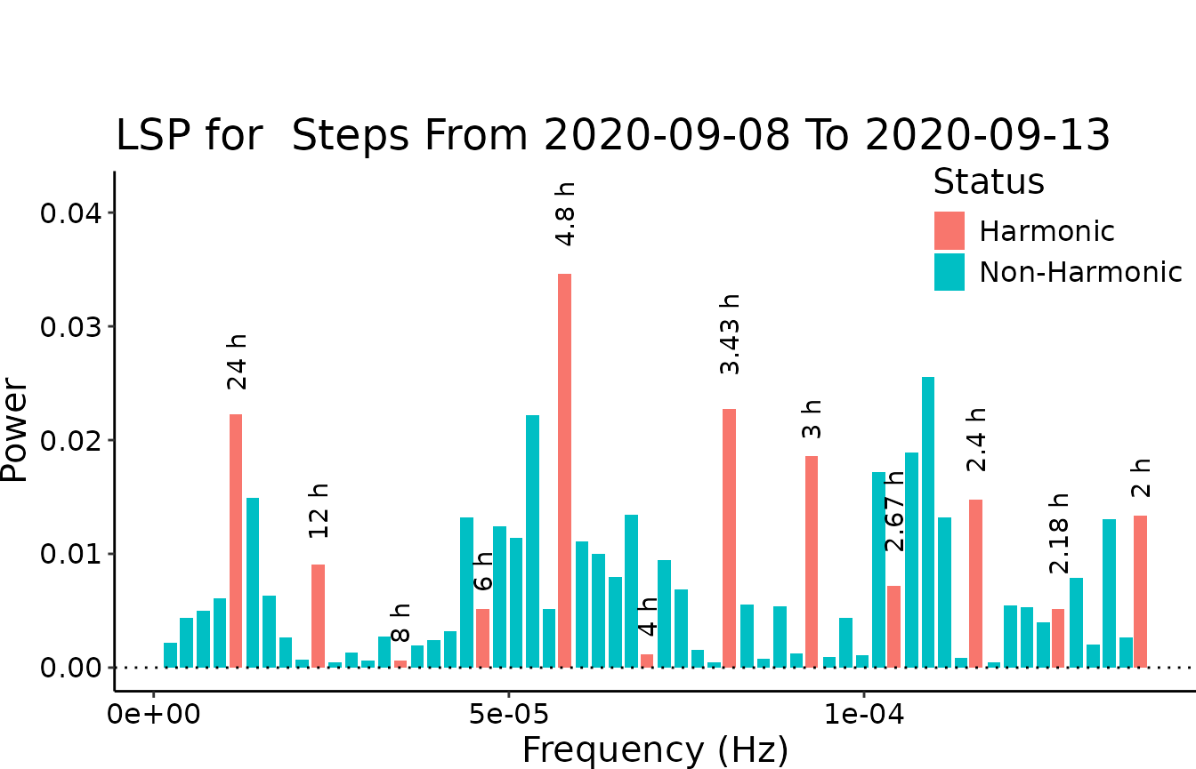
#> v Correct time format: First column has a POSIXct Format
#> v Number of days good for DFC: 5 days >= 2 days
#> v Correct numeric format - Column 2 ==> Steps
#> The data is digiRhythm friendly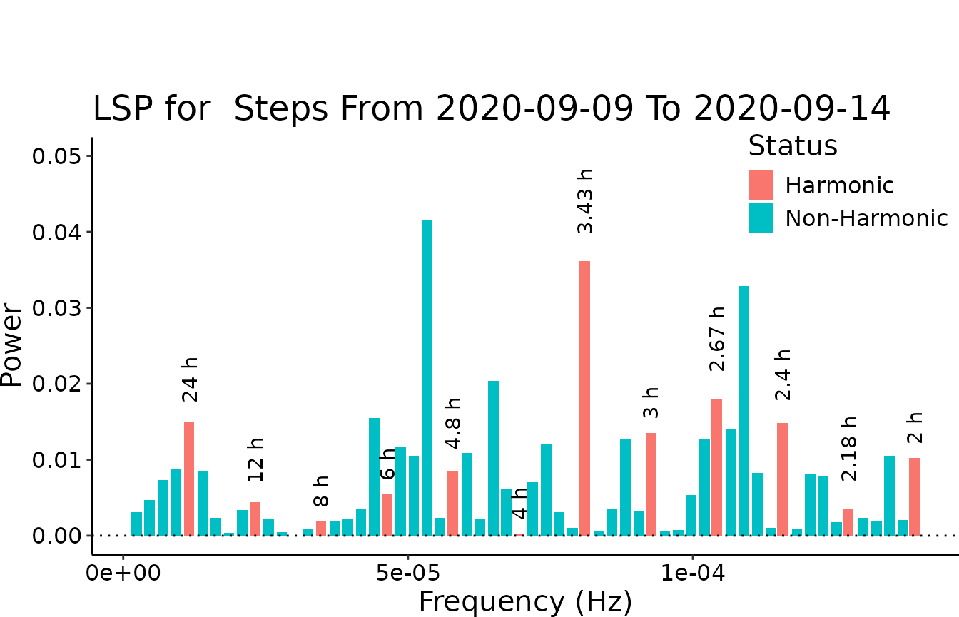
#> v Correct time format: First column has a POSIXct Format
#> v Number of days good for DFC: 5 days >= 2 days
#> v Correct numeric format - Column 2 ==> Steps
#> The data is digiRhythm friendly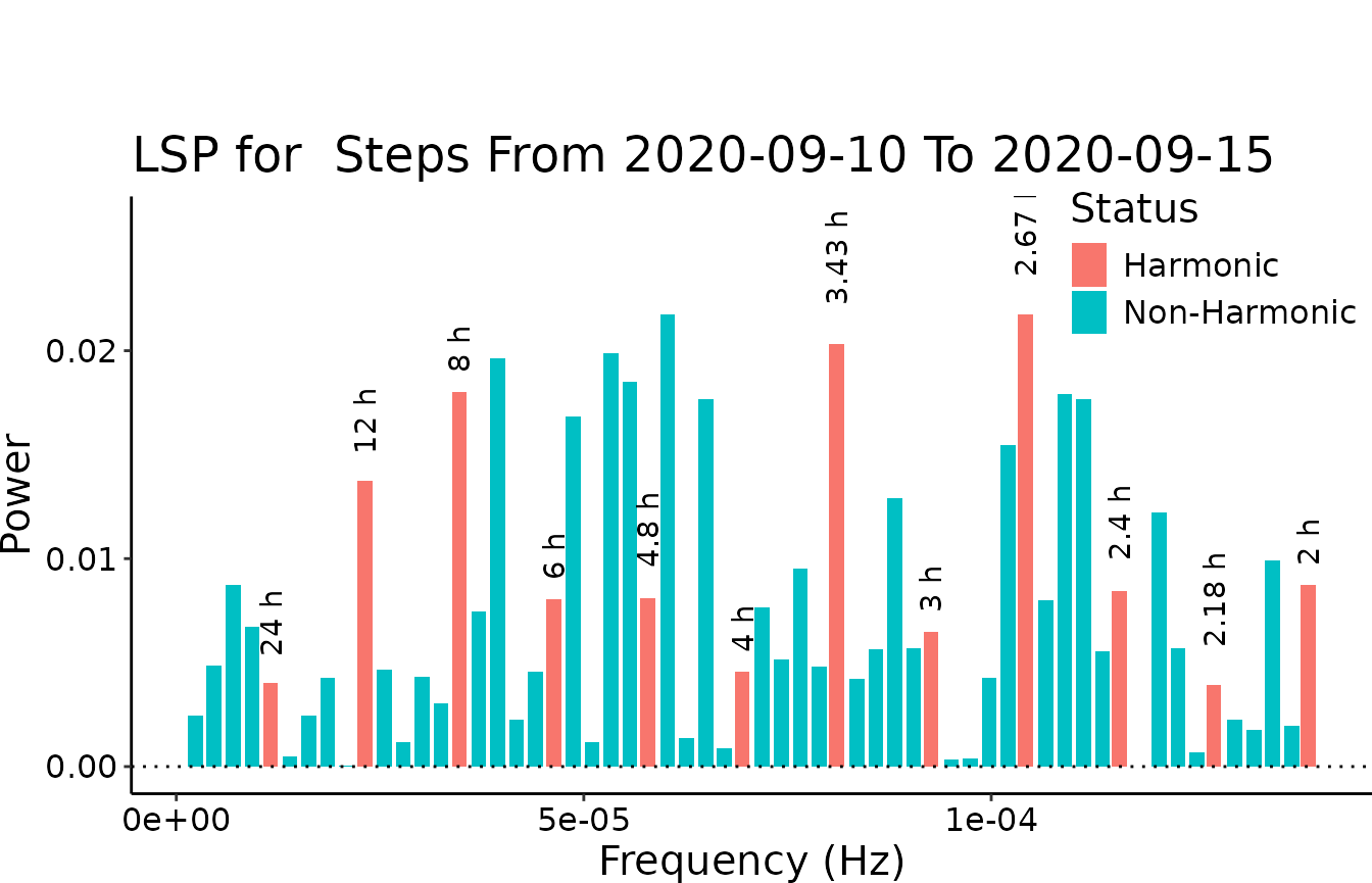
#> v Correct time format: First column has a POSIXct Format
#> v Number of days good for DFC: 5 days >= 2 days
#> v Correct numeric format - Column 2 ==> Steps
#> The data is digiRhythm friendly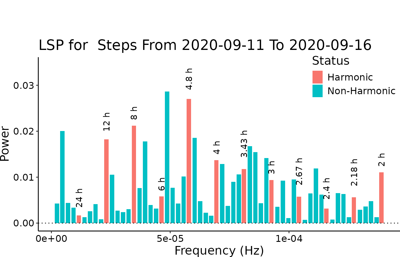
#> v Correct time format: First column has a POSIXct Format
#> v Number of days good for DFC: 5 days >= 2 days
#> v Correct numeric format - Column 2 ==> Steps
#> The data is digiRhythm friendly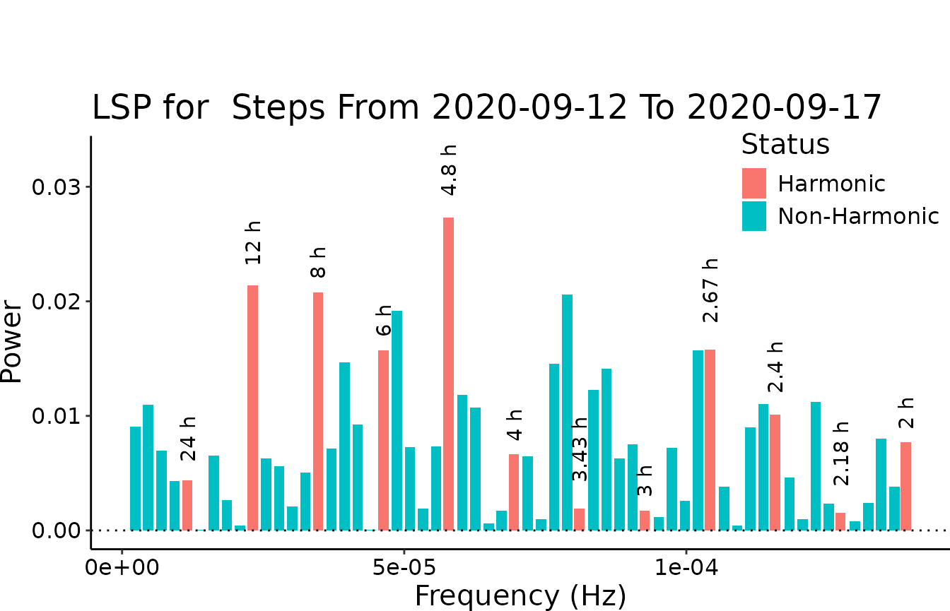
#> v Correct time format: First column has a POSIXct Format
#> v Number of days good for DFC: 5 days >= 2 days
#> v Correct numeric format - Column 2 ==> Steps
#> The data is digiRhythm friendly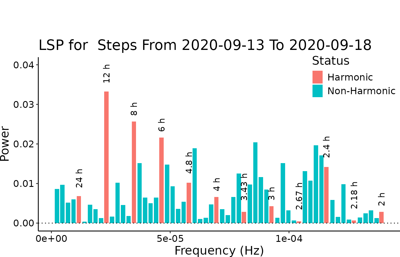
#> v Correct time format: First column has a POSIXct Format
#> v Number of days good for DFC: 5 days >= 2 days
#> v Correct numeric format - Column 2 ==> Steps
#> The data is digiRhythm friendly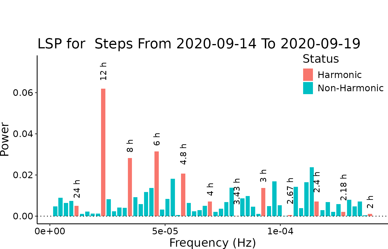
#> v Correct time format: First column has a POSIXct Format
#> v Number of days good for DFC: 5 days >= 2 days
#> v Correct numeric format - Column 2 ==> Steps
#> The data is digiRhythm friendly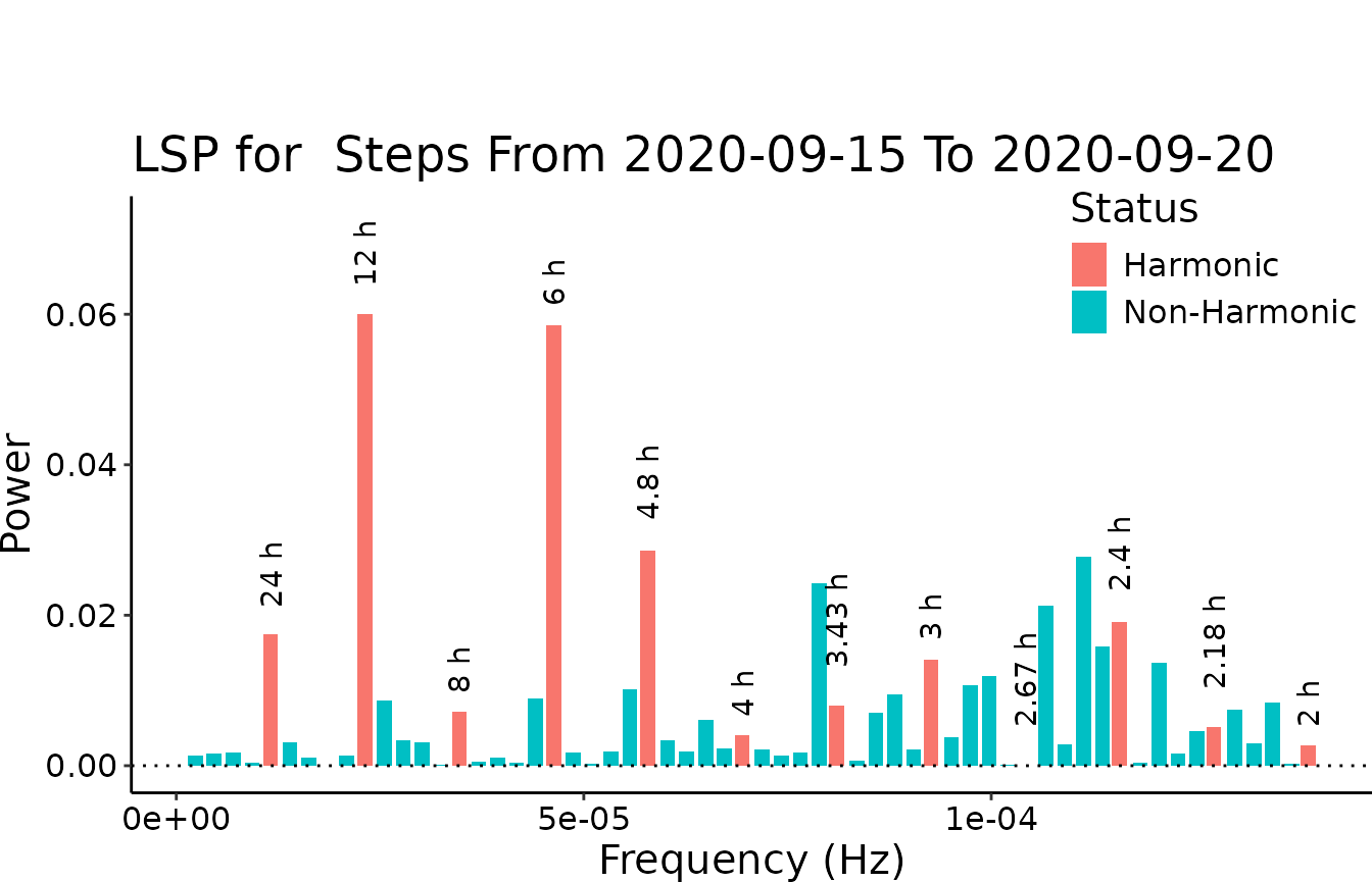
#> v Correct time format: First column has a POSIXct Format
#> v Number of days good for DFC: 5 days >= 2 days
#> v Correct numeric format - Column 2 ==> Steps
#> The data is digiRhythm friendly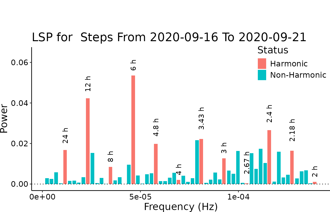
#> v Correct time format: First column has a POSIXct Format
#> v Number of days good for DFC: 5 days >= 2 days
#> v Correct numeric format - Column 2 ==> Steps
#> The data is digiRhythm friendly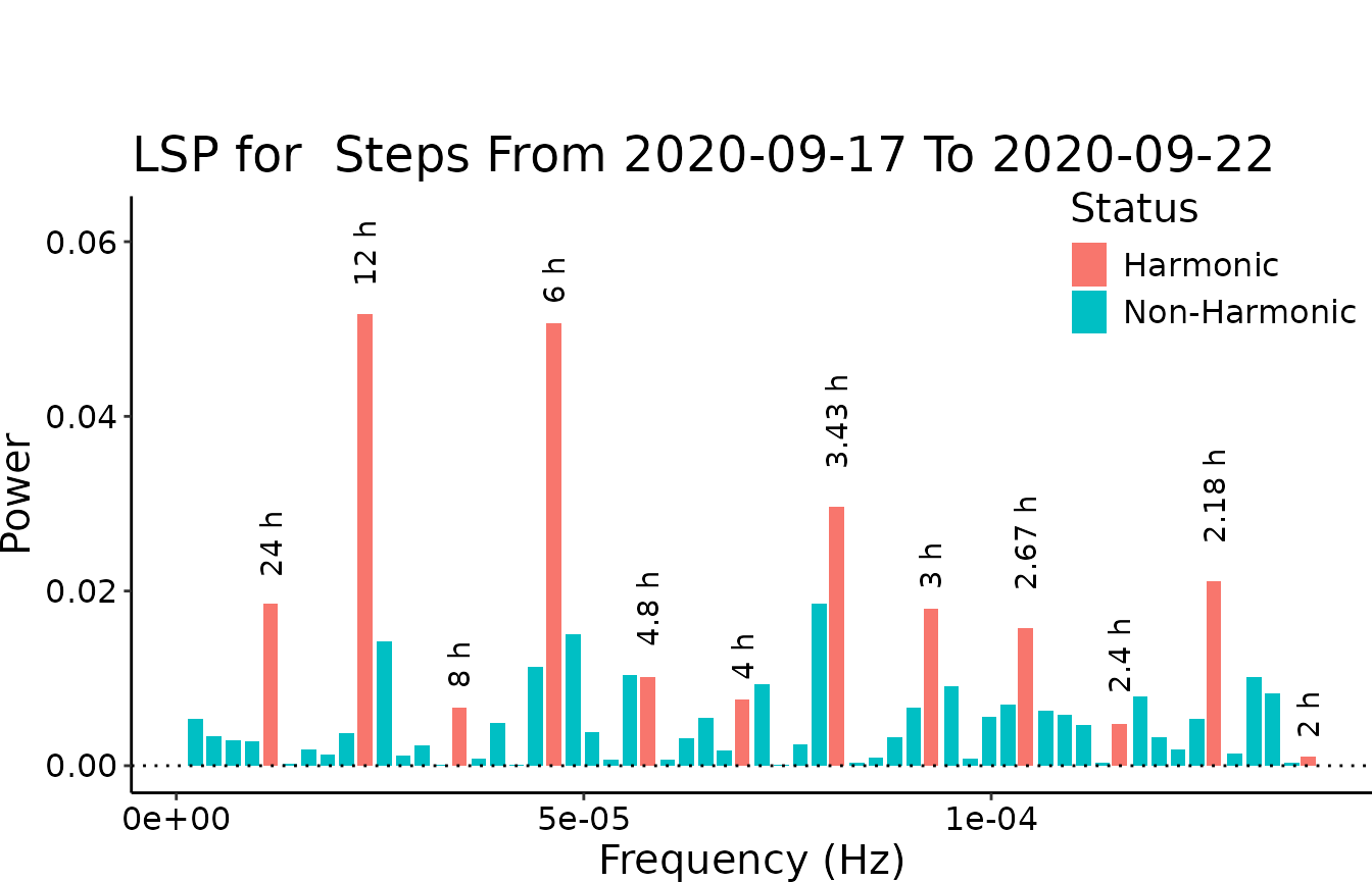
#> v Correct time format: First column has a POSIXct Format
#> v Number of days good for DFC: 5 days >= 2 days
#> v Correct numeric format - Column 2 ==> Steps
#> The data is digiRhythm friendly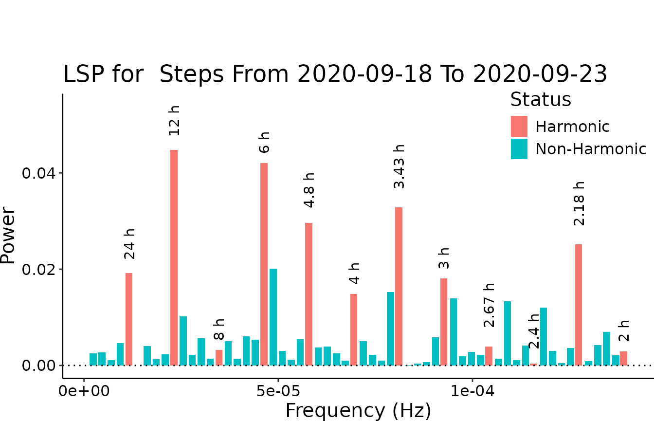
#> v Correct time format: First column has a POSIXct Format
#> v Number of days good for DFC: 5 days >= 2 days
#> v Correct numeric format - Column 2 ==> Steps
#> The data is digiRhythm friendly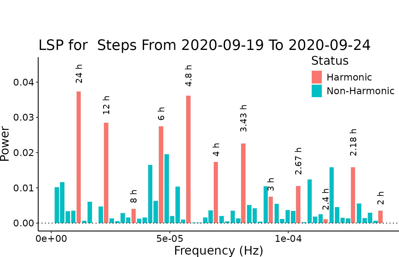
#> v Correct time format: First column has a POSIXct Format
#> v Number of days good for DFC: 5 days >= 2 days
#> v Correct numeric format - Column 2 ==> Steps
#> The data is digiRhythm friendly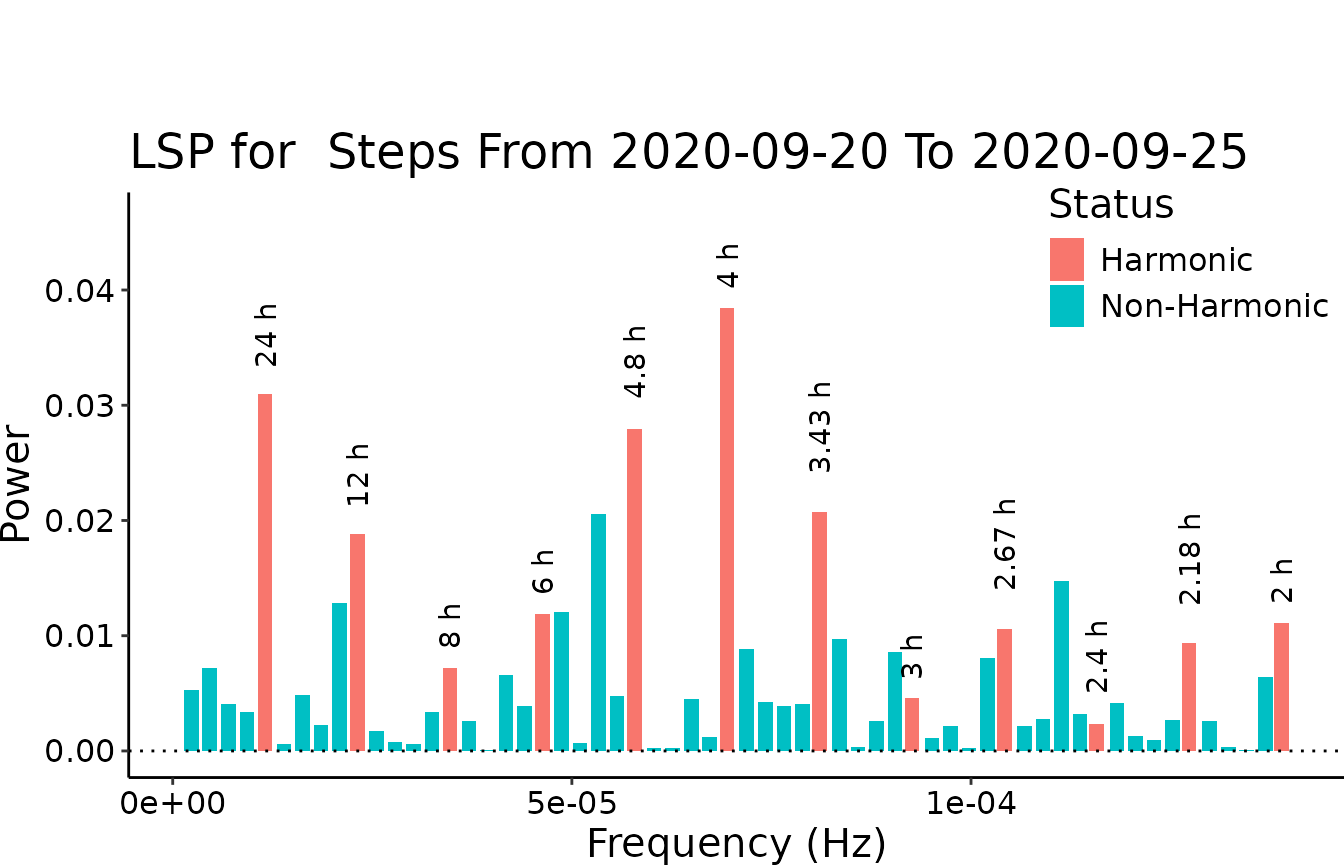
#> v Correct time format: First column has a POSIXct Format
#> v Number of days good for DFC: 5 days >= 2 days
#> v Correct numeric format - Column 2 ==> Steps
#> The data is digiRhythm friendly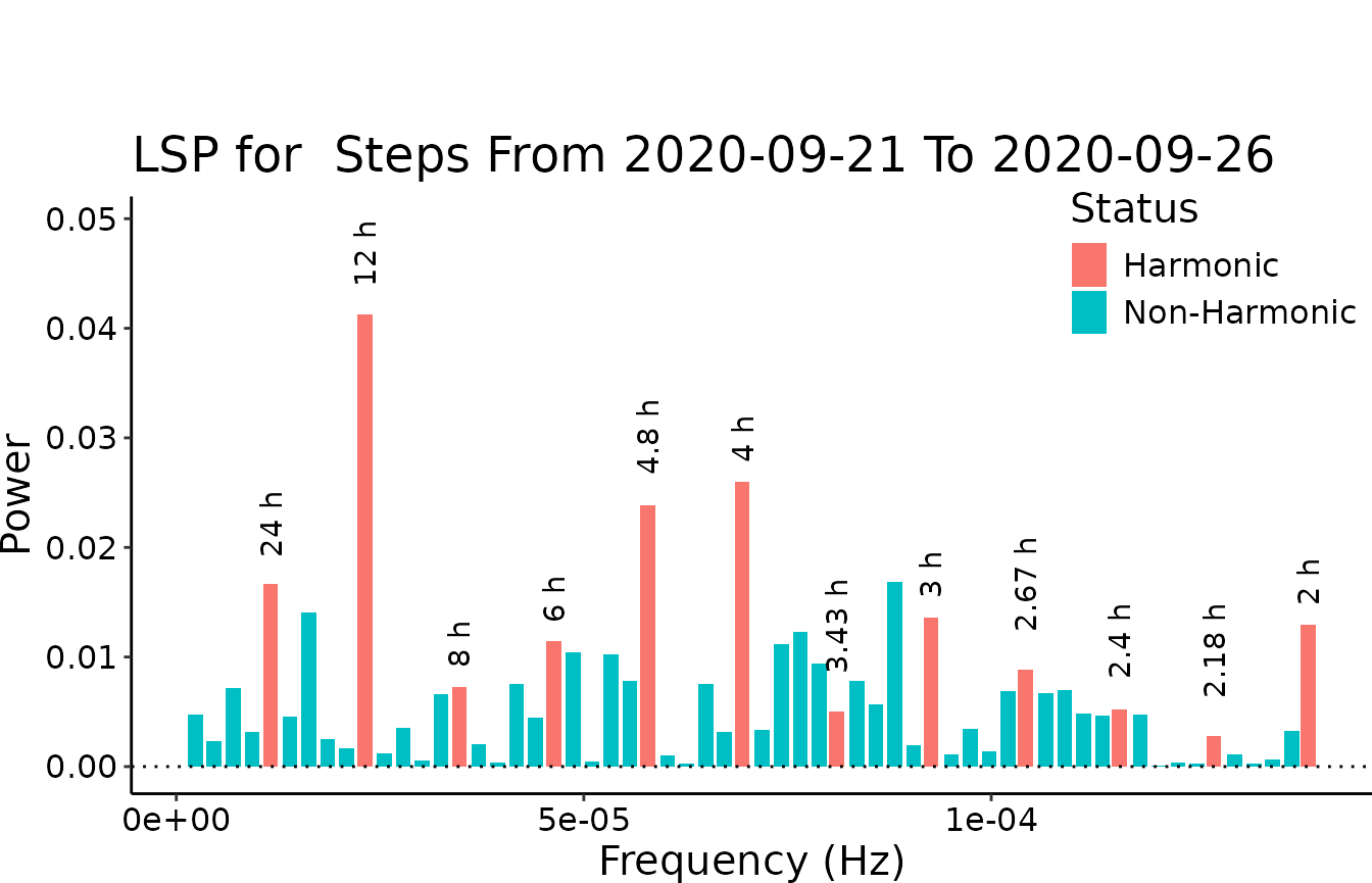
#> v Correct time format: First column has a POSIXct Format
#> v Number of days good for DFC: 5 days >= 2 days
#> v Correct numeric format - Column 2 ==> Steps
#> The data is digiRhythm friendly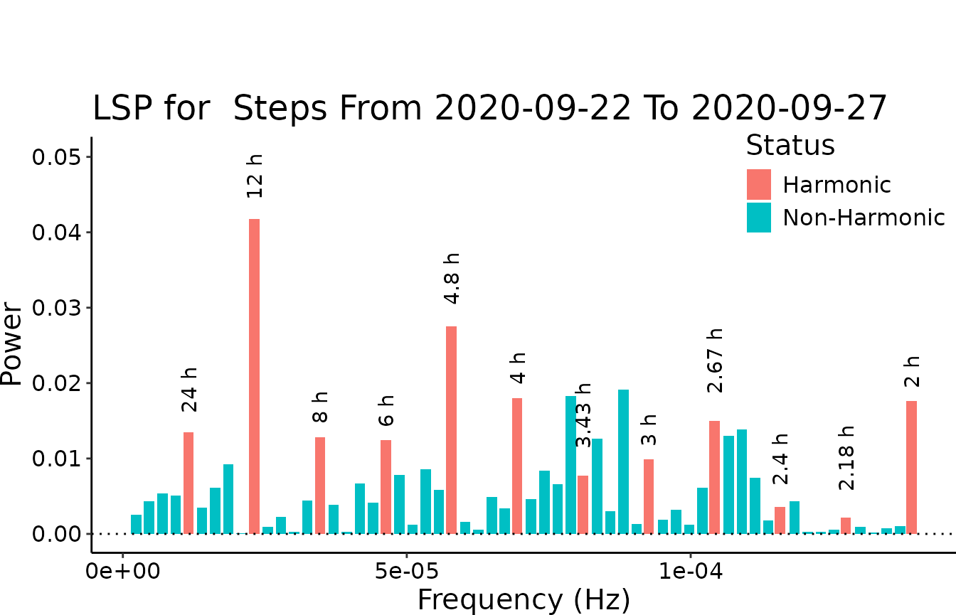
#> v Correct time format: First column has a POSIXct Format
#> v Number of days good for DFC: 5 days >= 2 days
#> v Correct numeric format - Column 2 ==> Steps
#> The data is digiRhythm friendly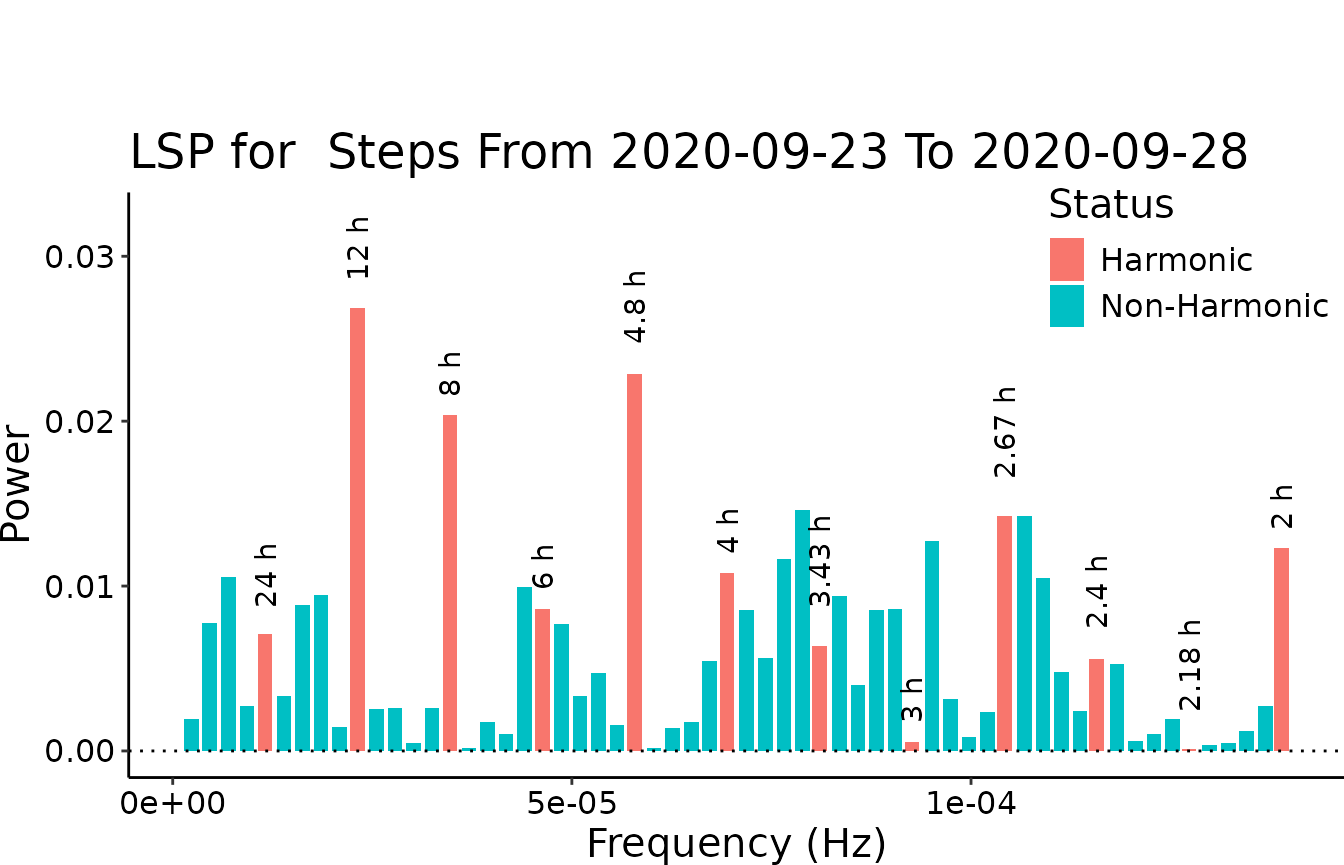
#> v Correct time format: First column has a POSIXct Format
#> v Number of days good for DFC: 5 days >= 2 days
#> v Correct numeric format - Column 2 ==> Steps
#> The data is digiRhythm friendly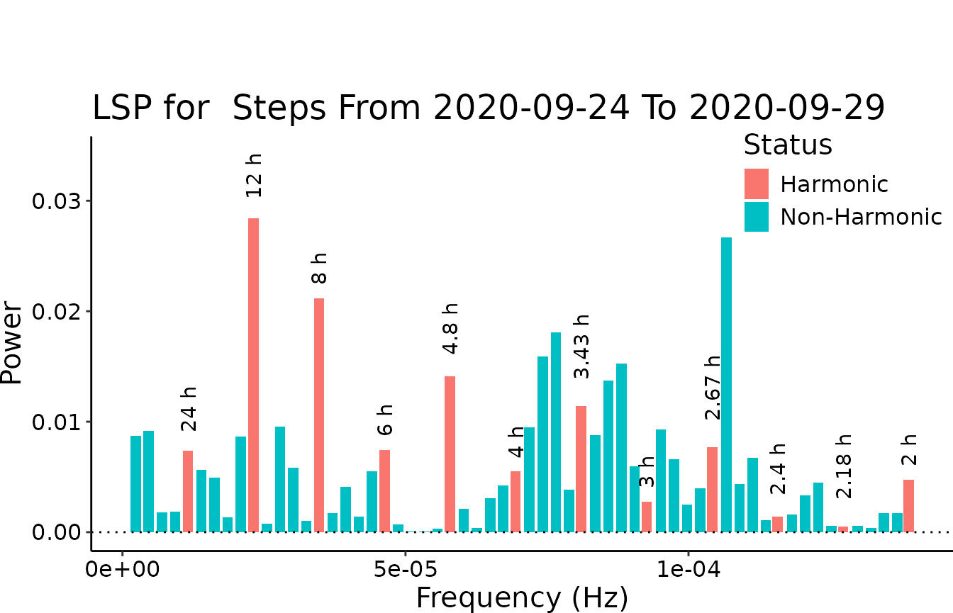
#> v Correct time format: First column has a POSIXct Format
#> v Number of days good for DFC: 5 days >= 2 days
#> v Correct numeric format - Column 2 ==> Steps
#> The data is digiRhythm friendly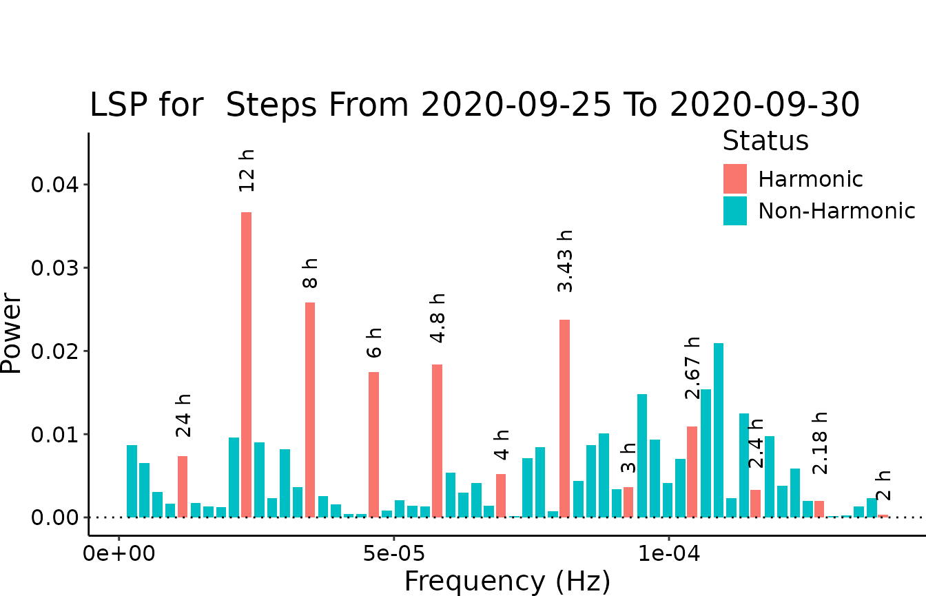
#> v Correct time format: First column has a POSIXct Format
#> v Number of days good for DFC: 5 days >= 2 days
#> v Correct numeric format - Column 2 ==> Steps
#> The data is digiRhythm friendly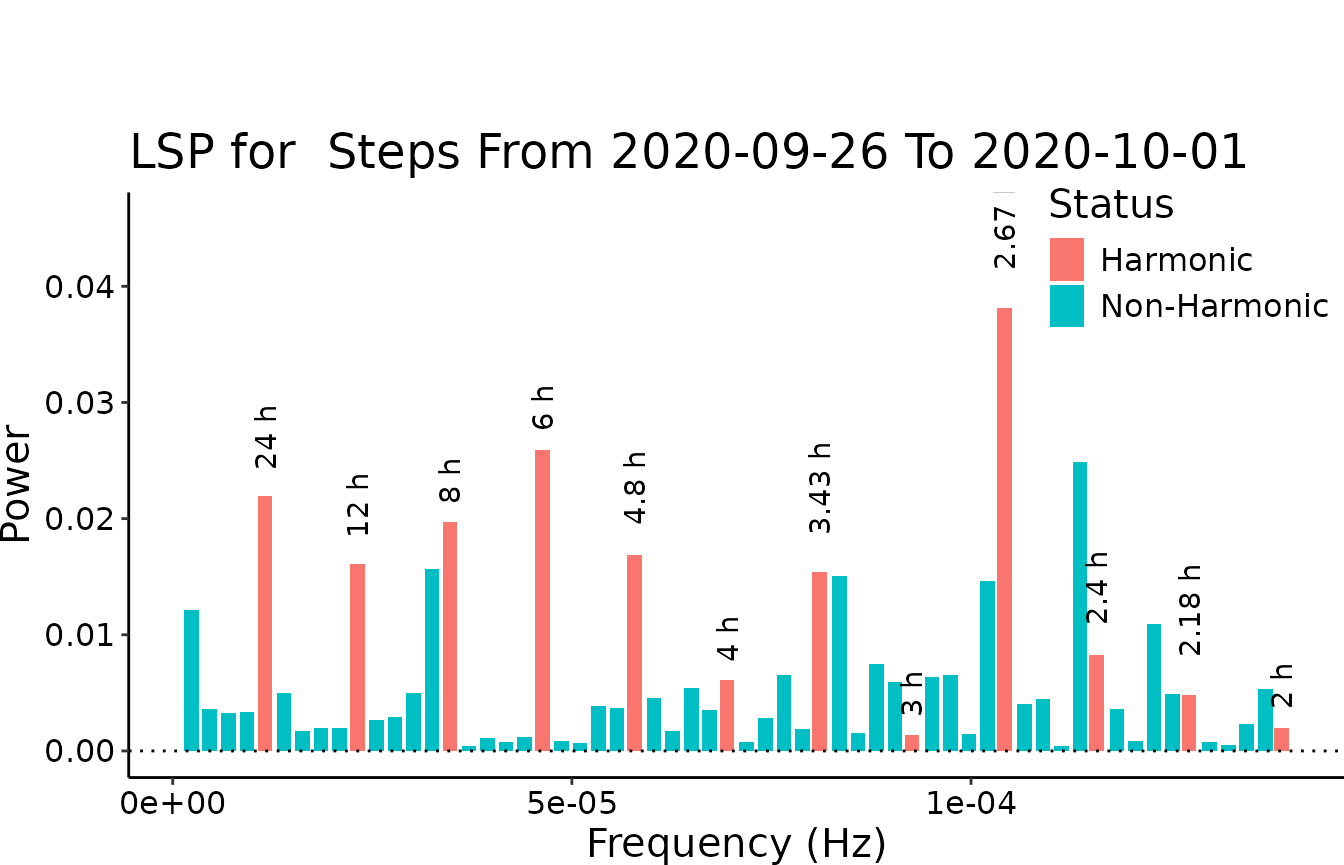
#> v Correct time format: First column has a POSIXct Format
#> v Number of days good for DFC: 5 days >= 2 days
#> v Correct numeric format - Column 2 ==> Steps
#> The data is digiRhythm friendly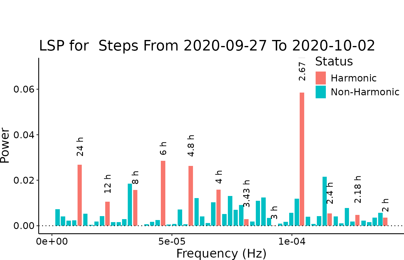
#> v Correct time format: First column has a POSIXct Format
#> v Number of days good for DFC: 5 days >= 2 days
#> v Correct numeric format - Column 2 ==> Steps
#> The data is digiRhythm friendly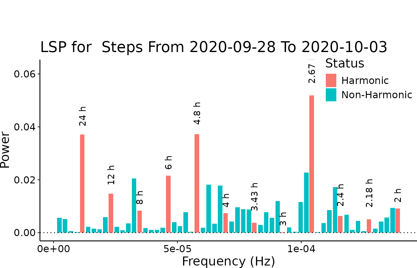
#> v Correct time format: First column has a POSIXct Format
#> v Number of days good for DFC: 5 days >= 2 days
#> v Correct numeric format - Column 2 ==> Steps
#> The data is digiRhythm friendly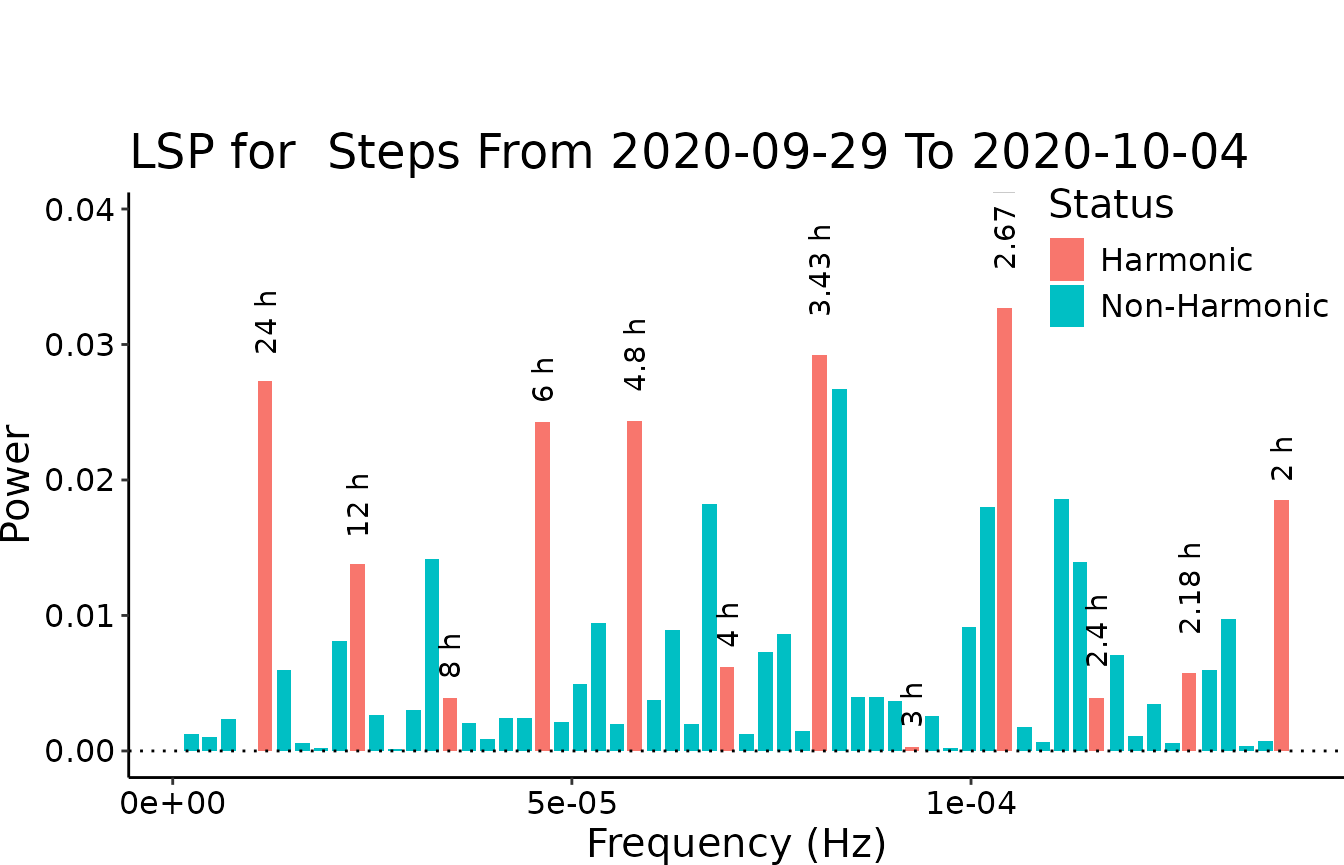
#> v Correct time format: First column has a POSIXct Format
#> v Number of days good for DFC: 5 days >= 2 days
#> v Correct numeric format - Column 2 ==> Steps
#> The data is digiRhythm friendly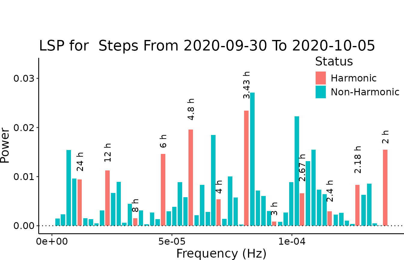
#> v Correct time format: First column has a POSIXct Format
#> v Number of days good for DFC: 5 days >= 2 days
#> v Correct numeric format - Column 2 ==> Steps
#> The data is digiRhythm friendly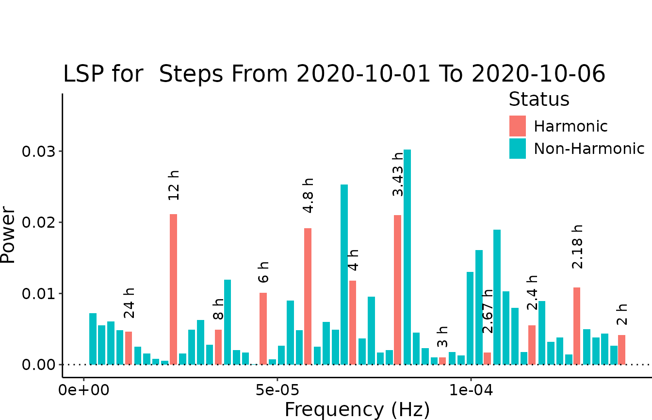
#> v Correct time format: First column has a POSIXct Format
#> v Number of days good for DFC: 5 days >= 2 days
#> v Correct numeric format - Column 2 ==> Steps
#> The data is digiRhythm friendly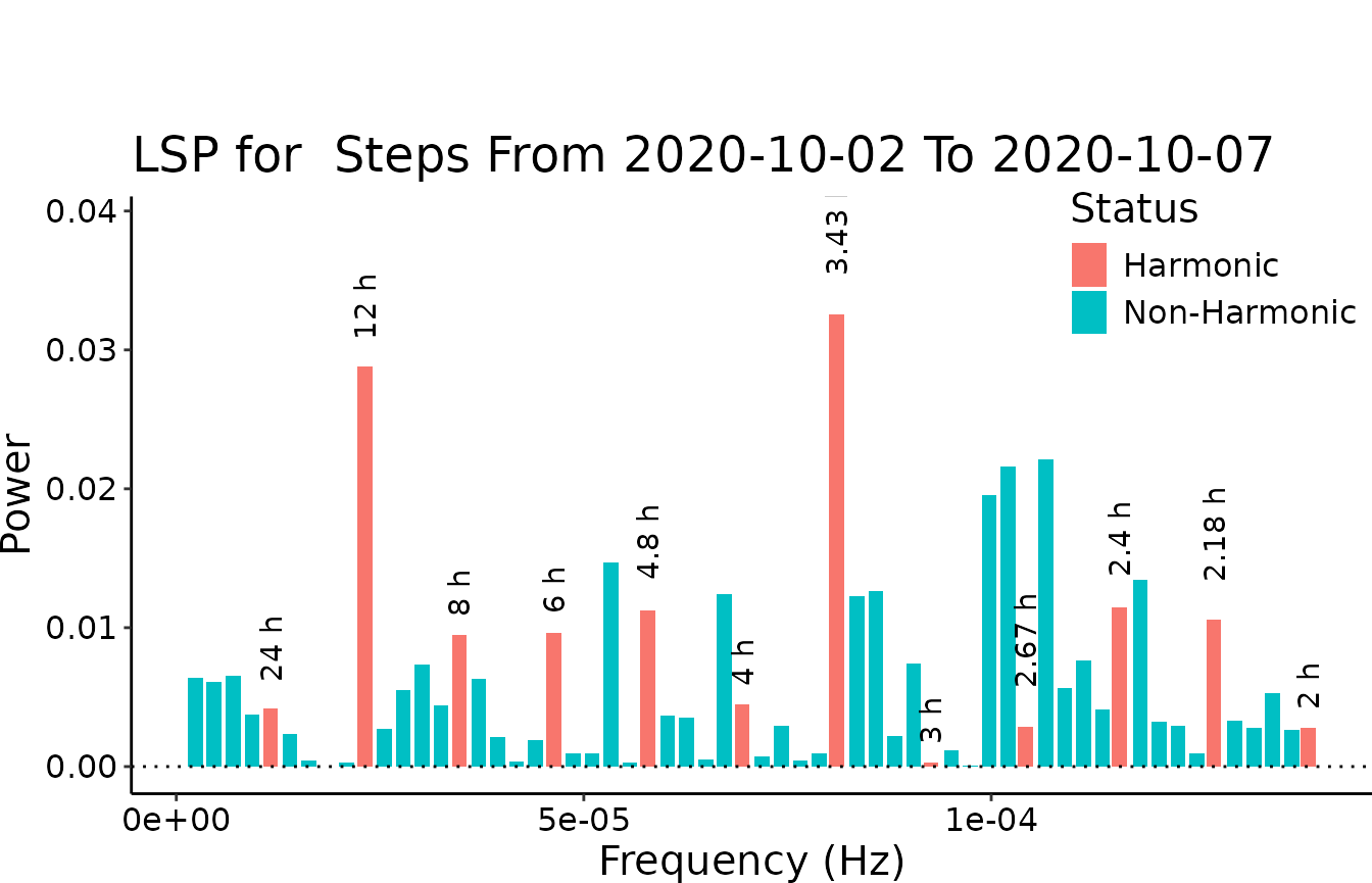
#> v Correct time format: First column has a POSIXct Format
#> v Number of days good for DFC: 5 days >= 2 days
#> v Correct numeric format - Column 2 ==> Steps
#> The data is digiRhythm friendly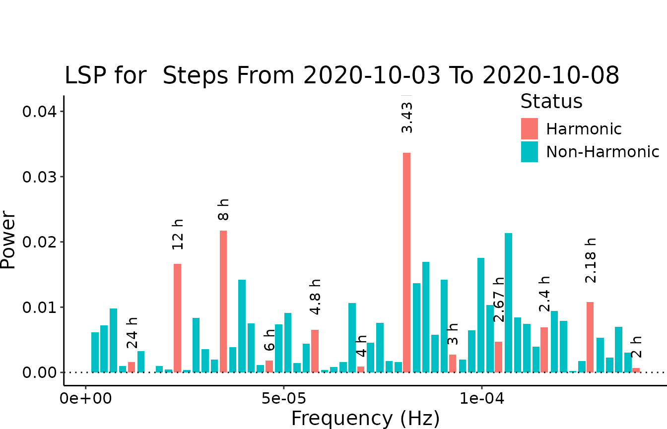
#> v Correct time format: First column has a POSIXct Format
#> v Number of days good for DFC: 5 days >= 2 days
#> v Correct numeric format - Column 2 ==> Steps
#> The data is digiRhythm friendly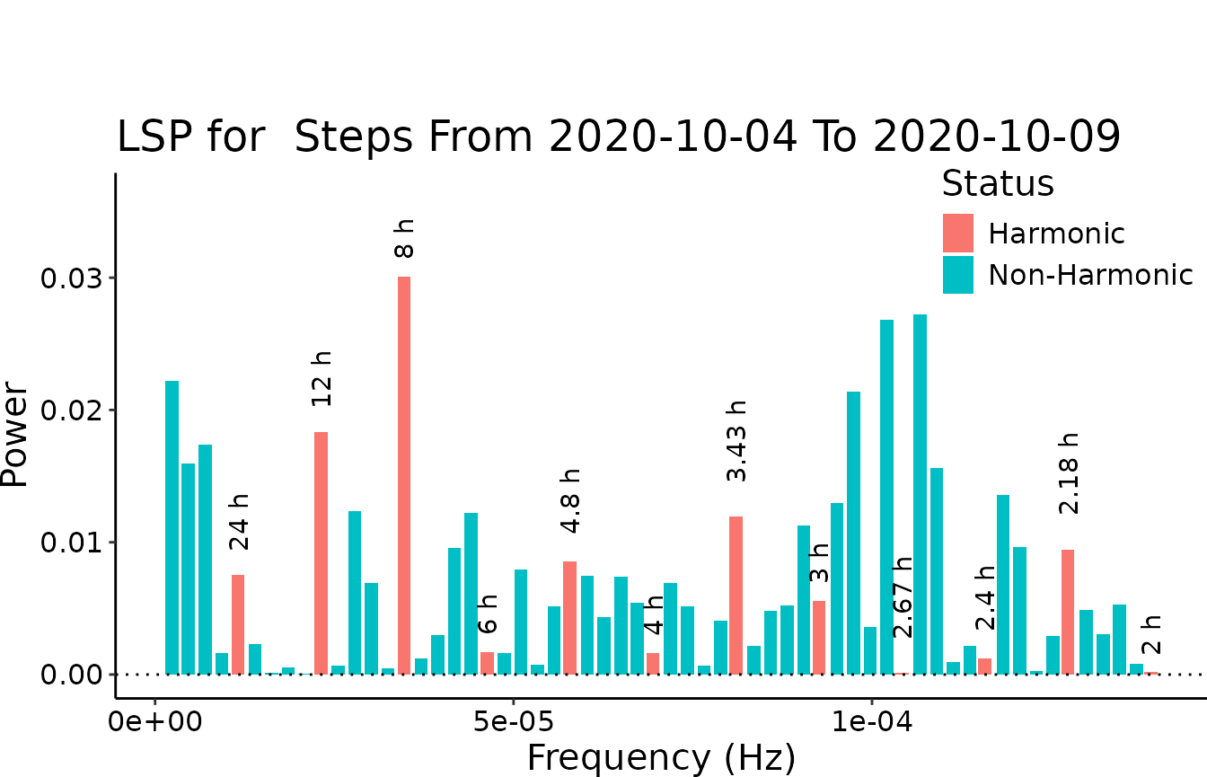
#> v Correct time format: First column has a POSIXct Format
#> v Number of days good for DFC: 5 days >= 2 days
#> v Correct numeric format - Column 2 ==> Steps
#> The data is digiRhythm friendly
# Setting plot to TRUE will visualize all the LSP plots (like the one above)
# during each sliding window. Rather used for deeper investigation and
# debugging.
print(my_dfc)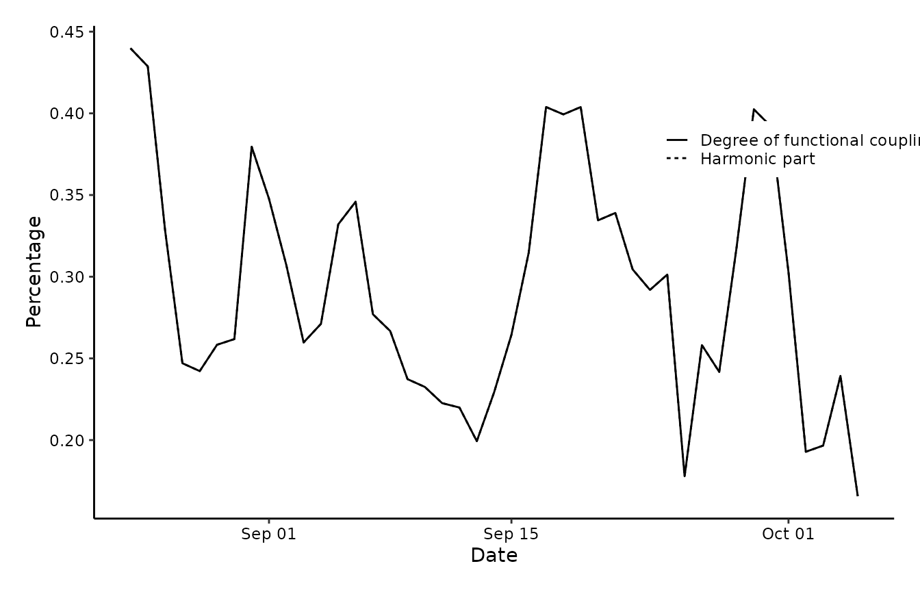 # Accessing output data and changing the plots using DigiRhythm
The DFC function returns a object of type ggplot:
class(my_dfc)
#> [1] "gg"     "ggplot"
As shown, the class is gg or ggplot. This allows the user to: - Access the data of DFC or HP directly from the returned object. - Add aesthetics layer to the plot as needed.
To access the data, user has to use the data component of the DFC object. We illustrate this in the below code:
head(my_dfc$data)
#>         from         to       dfc        hp
#> 1 2020-08-24 2020-08-28 0.4398348 0.4398348
#> 2 2020-08-25 2020-08-29 0.4287425 0.4287425
#> 3 2020-08-26 2020-08-30 0.3283561 0.3283561
#> 4 2020-08-27 2020-08-31 0.2470351 0.2470351
#> 5 2020-08-28 2020-09-01 0.2422273 0.2422273
#> 6 2020-08-29 2020-09-02 0.2583468 0.2583468
As shown, we can access a dataframe where the first comlumn is the date and the second two columns are the DFC and HP respectively. This will allow the users to be able to use the returned data in further studies such as modelling.
Users can also change the aesthetics of the plot directly if they wish. This is possible by adding a ggplot layer to the returned DFC object. For instance, this is the original plot returned by the DFC:
print(my_dfc)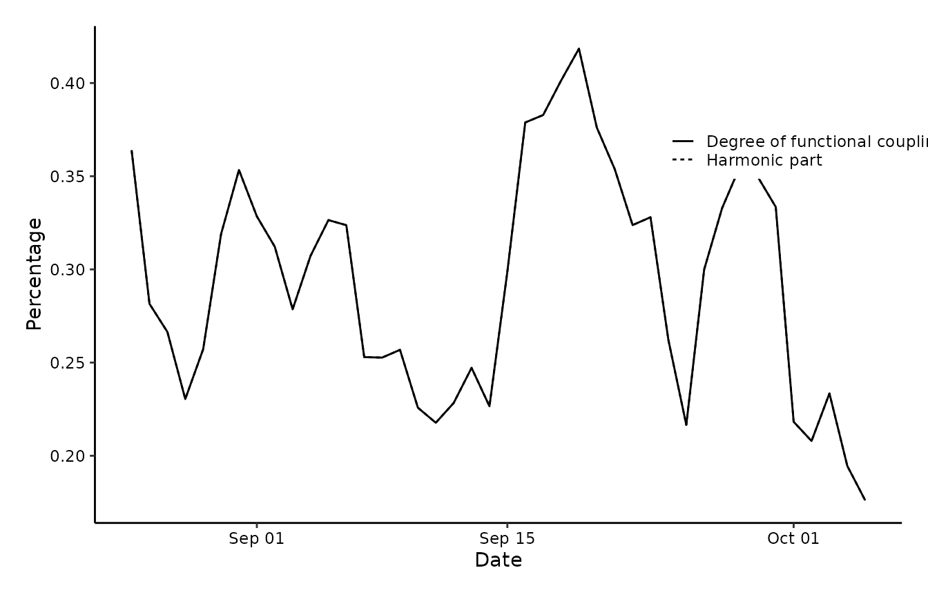 As an illustrative example, in the below code we add a new aesthetic
layer to the ggplot object. This layer does nothing but increasing the
width of the x-axis. Users can add any other aesthetic layer as they
wish; the immagination is the only limit.
library(ggplot2)
new_plot <- my_dfc +
  theme(
    text = element_text(family = "Times", size = 14),
    axis.text.y = element_text(size = 15, colour = "black")
  )
print(new_plot)